Linear Regression
// Line of Best Fit
SciKit-Learn
Note: number of iterations and learning rate are preset, I don't know how you can change them...
Import
from sklearn.linear_model import LinearRegressionFit data
line_fitter = LinearRegression()

# x and y are lists
line_fitter.fit(x, y)


# get slope
line_fitter.coef_

# get intercept
line_fitter.intercept_
Predict
# takes in a list of x, returns a list of y
y_predicted = line_fitter.predict(x)
Loss

This is how we decide how far off the line is, from being best fit
This is done by; getting the squared distance of each point from the line
The distance is squared so there all positive (contribute in the same way)
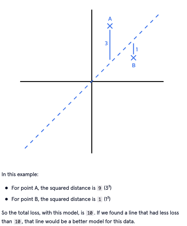
Loss is found by:
- Getting the difference between Y and predictedY
- Squaring the difference
- Adding it to total loss
Example code
#data
x = [1, 2, 3]
y = [5, 1, 3]


#y = x
m1 = 1
b1 = 0

y_predicted1 = []

for i in x:
  y_predicted1.append(i)

total_loss1 = 0

for i in range(len(y_predicted1)):
  total_loss1 += (y_predicted1[i] - y[i]) ** 2


#y = 0.5x + 1
m2 = 0.5
b2 = 1

y_predicted2 = []

for i in x:
  y_predicted2.append(i * 0.5 + 1)

total_loss2 = 0

for i in range(len(y_predicted2)):
  total_loss2 += (y_predicted2[i] - y[i]) ** 2


#determining the better fit

print(total_loss1)
print(total_loss2)

if total_loss1 < total_loss2:
  better_fit = 1
else:
  better_fit = 2
Gradient Descent
Goal get to the minimum loss
The process is Gradient Decent
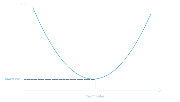
For Intercept (B and M)
Note: this works for both finding the loss with both M and B,
no change to the formula required
RETURNS gradient with our guessed M and B values, on the graph above, goal is to get 0
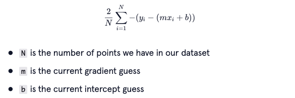
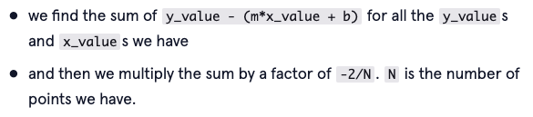
Code for the formula
def get_gradient_at_b(x, y, m, b):
  diff = 0

  for i in range(len(y)):
    diff += (y[i] - ((m * x[i]) + b))

  b_gradient = (-2/len(y)) * diff

  return b_gradient
Gradient Step
This is how large each step we make is towards the lowest loss.
#to find a new b value
new_b = current_b - (learning_rate * b_gradient)
# note that as we get closer to 0 (the goal)
# our steps get smaller and smaller
A full function
def step_gradient(x, y, b_current, m_current):

  b_gradient = get_gradient_at_b(x, y, b_current, m_current)
  m_gradient = get_gradient_at_m(x, y, b_current, m_current)

  b = b_current - (0.01 * b_gradient)
  m = m_current - (0.01 * m_gradient)

  return (b, m)
Note: for the code to work we need to call this loads
Convergence and Learning Rate
Convergence refers to when the parameters stop changing with each iteration.
Learning rate refers to how much the parameters are changed on each iteration.
The gains from calling the function will get smaller and smaller
This bit is how we know when to stop spamming the function
And how big or small the steps need to be, or else we might spend too long searching
Example code
this code follows from the code shown above
#Your gradient_descent function here:
def gradient_descent(x, y, learning_rate, num_iterations):
  b = 0
  m = 0

  for i in range(num_iterations):
    b, m = step_gradient(b, m, x, y, learning_rate)

  return [b, m]

#data
months = [1, 2, 3, 4, 5, 6, 7, 8, 9, 10, 11, 12]
revenue = [52, 74, 79, 95, 115, 110, 129, 126, 147, 146, 156, 184]

#calling the function
b, m = gradient_descent(months, revenue, 0.01, 1000)

#showing the data on a graph
y = [m*x + b for x in months]

plt.plot(months, revenue, "o")
plt.plot(months, y)

plt.show()